🌽 Crop Classification and Clustering

import numpy as np 
import pandas as pd 
import matplotlib.pyplot as plt
import seaborn as sns
import matplotlib.gridspec as gridspec
import math

## Models
from sklearn.linear_model import LogisticRegression
from sklearn.neighbors import KNeighborsClassifier
from sklearn.ensemble import RandomForestClassifier
from sklearn.ensemble import GradientBoostingClassifier
from sklearn.naive_bayes import GaussianNB

from sklearn.model_selection import train_test_split
from sklearn.model_selection import RandomizedSearchCV, GridSearchCV
from sklearn.metrics import confusion_matrix, classification_report, accuracy_score
from sklearn.metrics import precision_score, recall_score, f1_score

from sklearn.impute import SimpleImputer
from sklearn.compose import ColumnTransformer
from sklearn.pipeline import Pipeline
from sklearn.preprocessing import StandardScaler

EDA

df = pd.read_csv('Crop_Recommendation.csv')
df

	Nitrogen	Phosphorus	Potassium	Temperature	Humidity	pH_Value	Rainfall	Crop
0	90	42	43	20.879744	82.002744	6.502985	202.935536	Rice
1	85	58	41	21.770462	80.319644	7.038096	226.655537	Rice
2	60	55	44	23.004459	82.320763	7.840207	263.964248	Rice
3	74	35	40	26.491096	80.158363	6.980401	242.864034	Rice
4	78	42	42	20.130175	81.604873	7.628473	262.717340	Rice
...	...	...	...	...	...	...	...	...
2195	107	34	32	26.774637	66.413269	6.780064	177.774507	Coffee
2196	99	15	27	27.417112	56.636362	6.086922	127.924610	Coffee
2197	118	33	30	24.131797	67.225123	6.362608	173.322839	Coffee
2198	117	32	34	26.272418	52.127394	6.758793	127.175293	Coffee
2199	104	18	30	23.603016	60.396475	6.779833	140.937041	Coffee

2200 rows × 8 columns

features = df.columns[:-1]
features

Index(['Nitrogen', 'Phosphorus', 'Potassium', 'Temperature', 'Humidity',
       'pH_Value', 'Rainfall'],
      dtype='object')

df.Crop.nunique()

22

df.Crop.value_counts()

Crop
Rice           100
Maize          100
Jute           100
Cotton         100
Coconut        100
Papaya         100
Orange         100
Apple          100
Muskmelon      100
Watermelon     100
Grapes         100
Mango          100
Banana         100
Pomegranate    100
Lentil         100
Blackgram      100
MungBean       100
MothBeans      100
PigeonPeas     100
KidneyBeans    100
ChickPea       100
Coffee         100
Name: count, dtype: int64

df.Crop.value_counts(normalize=True)

Crop
Rice           0.045455
Maize          0.045455
Jute           0.045455
Cotton         0.045455
Coconut        0.045455
Papaya         0.045455
Orange         0.045455
Apple          0.045455
Muskmelon      0.045455
Watermelon     0.045455
Grapes         0.045455
Mango          0.045455
Banana         0.045455
Pomegranate    0.045455
Lentil         0.045455
Blackgram      0.045455
MungBean       0.045455
MothBeans      0.045455
PigeonPeas     0.045455
KidneyBeans    0.045455
ChickPea       0.045455
Coffee         0.045455
Name: proportion, dtype: float64

df.info()

<class 'pandas.core.frame.DataFrame'>
RangeIndex: 2200 entries, 0 to 2199
Data columns (total 8 columns):
 #   Column       Non-Null Count  Dtype  
---  ------       --------------  -----  
 0   Nitrogen     2200 non-null   int64  
 1   Phosphorus   2200 non-null   int64  
 2   Potassium    2200 non-null   int64  
 3   Temperature  2200 non-null   float64
 4   Humidity     2200 non-null   float64
 5   pH_Value     2200 non-null   float64
 6   Rainfall     2200 non-null   float64
 7   Crop         2200 non-null   object 
dtypes: float64(4), int64(3), object(1)
memory usage: 137.6+ KB

df.isna().sum()

Nitrogen       0
Phosphorus     0
Potassium      0
Temperature    0
Humidity       0
pH_Value       0
Rainfall       0
Crop           0
dtype: int64

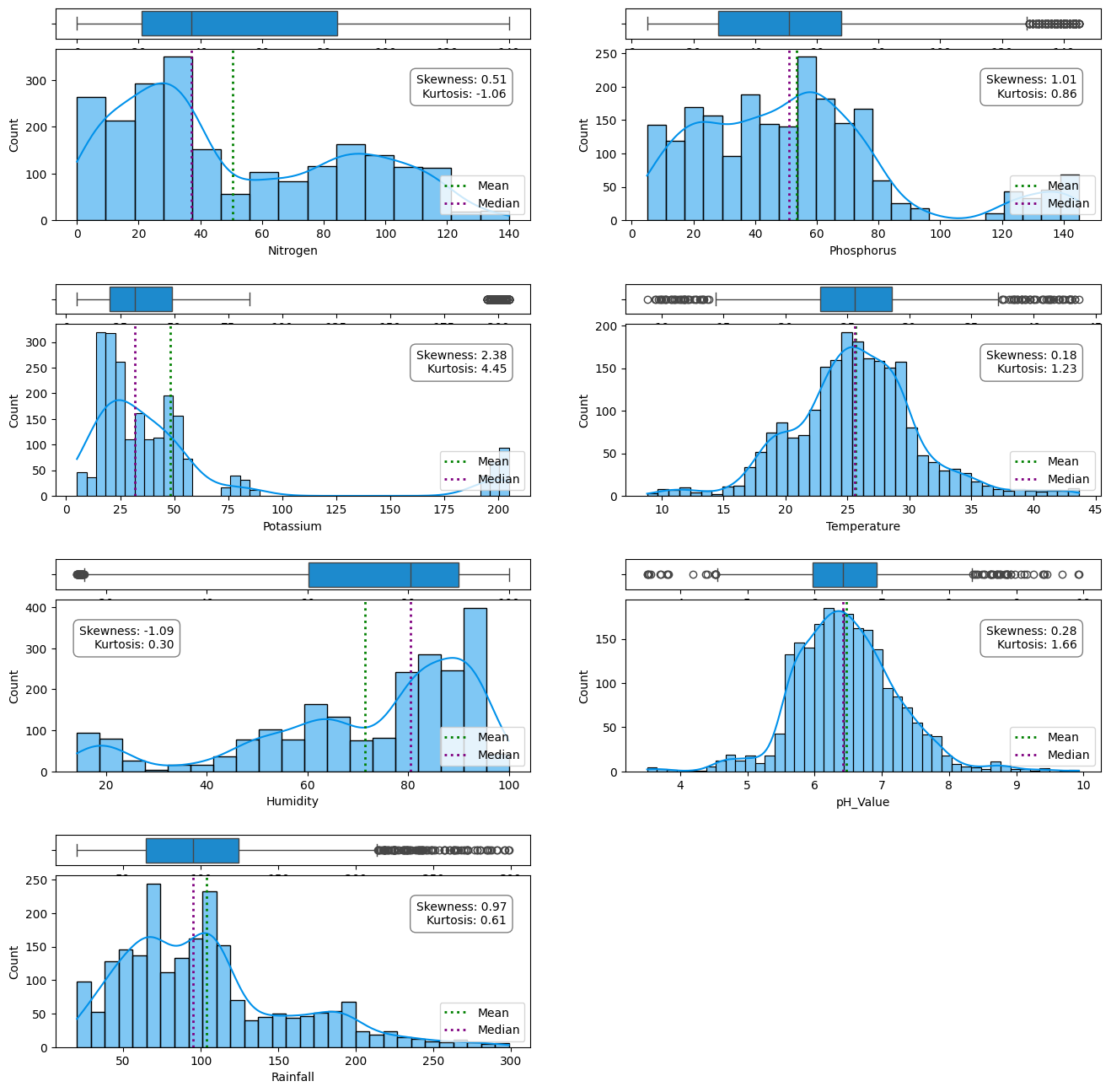
df.describe().T

	count	mean	std	min	25%	50%	75%	max
Nitrogen	2200.0	50.551818	36.917334	0.000000	21.000000	37.000000	84.250000	140.000000
Phosphorus	2200.0	53.362727	32.985883	5.000000	28.000000	51.000000	68.000000	145.000000
Potassium	2200.0	48.149091	50.647931	5.000000	20.000000	32.000000	49.000000	205.000000
Temperature	2200.0	25.616244	5.063749	8.825675	22.769375	25.598693	28.561654	43.675493
Humidity	2200.0	71.481779	22.263812	14.258040	60.261953	80.473146	89.948771	99.981876
pH_Value	2200.0	6.469480	0.773938	3.504752	5.971693	6.425045	6.923643	9.935091
Rainfall	2200.0	103.463655	54.958389	20.211267	64.551686	94.867624	124.267508	298.560117

Probably a good idea to standardize these values

# Correlation Matrix
corr_matrix = df.corr(numeric_only=True)
plt.figure(figsize=(15, 10))
sns.heatmap(corr_matrix, 
            annot=True, 
            linewidths=0.5, 
            fmt= ".2f", 
            cmap="YlGnBu");

metric_col = df.select_dtypes(include=['number']).columns

---

Modeling

X = df.drop('Crop', axis=1)
y = df.Crop.values

scaler = StandardScaler()
X = scaler.fit_transform(X)

# Train and Test Split
np.random.seed(42)

X_train, X_test, y_train, y_test = train_test_split(X,
                                                    y,
                                                    test_size=0.2)

X_train.shape, X_test.shape, y_train.shape, y_test.shape

((1760, 7), (440, 7), (1760,), (440,))

# Put models in a dictionary
models = {"KNN": KNeighborsClassifier(),
          "Logistic Regression": LogisticRegression(), 
          "Random Forest": RandomForestClassifier(),
          "GradientBoost": GradientBoostingClassifier(),
          "GaussianNB": GaussianNB(),
          }

# Create function to fit and score models
def fit_and_score(models, X_train, X_test, y_train, y_test):
    """
    Fits and evaluates given machine learning models.
    models : a dict of different Scikit-Learn machine learning models
    X_train : training data
    X_test : testing data
    y_train : labels assosciated with training data
    y_test : labels assosciated with test data
    """
    # Random seed for reproducible results
    np.random.seed(42)
    # Make a list to keep model scores
    model_scores = {}
    # Loop through models
    for name, model in models.items():
        # Fit the model to the data
        model.fit(X_train, y_train)
        # Evaluate the model and append its score to model_scores
        model_scores[name] = model.score(X_test, y_test)
    return model_scores

model_scores = fit_and_score(models=models,
                             X_train=X_train,
                             X_test=X_test,
                             y_train=y_train,
                             y_test=y_test)
model_scores

C:\Users\tuckerd9\AppData\Roaming\Python\Python39\site-packages\sklearn\linear_model\_logistic.py:444: ConvergenceWarning: lbfgs failed to converge (status=1):
STOP: TOTAL NO. of ITERATIONS REACHED LIMIT.

Increase the number of iterations (max_iter) or scale the data as shown in:
    https://scikit-learn.org/stable/modules/preprocessing.html
Please also refer to the documentation for alternative solver options:
    https://scikit-learn.org/stable/modules/linear_model.html#logistic-regression
  n_iter_i = _check_optimize_result(

{'KNN': 0.9568181818181818,
 'Logistic Regression': 0.9636363636363636,
 'Random Forest': 0.9931818181818182,
 'GradientBoost': 0.9818181818181818,
 'GaussianNB': 0.9954545454545455}

I could go with GaussianNB, but just choosing RandomForest model

model_compare = pd.DataFrame(model_scores, index=['accuracy'])
model_compare.T.plot.bar();

rf = RandomForestClassifier()
rf.fit(X_train, y_train)
y_preds_rf = rf.predict(X_test)

# Create a new dataframe with two columns: 'test' and 'predicted'
df_with_preds = pd.DataFrame({
    'test': y_test,
    'predicted': y_preds_rf
})
df_with_preds

	test	predicted
0	Muskmelon	Muskmelon
1	Watermelon	Watermelon
2	Papaya	Papaya
3	Papaya	Papaya
4	Apple	Apple
...	...	...
435	Rice	Rice
436	Rice	Rice
437	Cotton	Cotton
438	Cotton	Cotton
439	PigeonPeas	PigeonPeas

440 rows × 2 columns

# Create a new dataframe with the predicted values as a column
df_with_preds = pd.DataFrame(X_test, columns=X_test.columns)
df_with_preds['actual'] = y_test
df_with_preds['predicted'] = y_preds_rf
df_with_preds

	Nitrogen	Phosphorus	Potassium	Temperature	Humidity	pH_Value	Rainfall	actual	predicted
1451	101	17	47	29.494014	94.729813	6.185053	26.308209	Muskmelon	Muskmelon
1334	98	8	51	26.179346	86.522581	6.259336	49.430510	Watermelon	Watermelon
1761	59	62	49	43.360515	93.351916	6.941497	114.778071	Papaya	Papaya
1735	44	60	55	34.280461	90.555616	6.825371	98.540477	Papaya	Papaya
1576	30	137	200	22.914300	90.704756	5.603413	118.604465	Apple	Apple
...	...	...	...	...	...	...	...	...	...
59	99	55	35	21.723831	80.238990	6.501698	277.962619	Rice	Rice
71	67	45	38	22.727910	82.170688	7.300411	260.887506	Rice	Rice
1908	121	47	16	23.605640	79.295731	7.723240	72.498009	Cotton	Cotton
1958	116	52	19	22.942767	75.371706	6.114526	67.080226	Cotton	Cotton
482	5	68	20	19.043805	33.106951	6.121667	155.370562	PigeonPeas	PigeonPeas

440 rows × 9 columns

def plot_confusion_matrix(y_test, predictions):
    # Plot the confusion matrix
    cf_matrix = confusion_matrix(y_test, predictions)
    fig = plt.subplots(figsize=(10, 8))
    sns.set(font_scale=1.4)
    sns.heatmap(cf_matrix, annot=True, fmt='d')
    plt.xlabel('Predicted Label', fontsize=12)
    plt.xticks(fontsize=12)
    plt.ylabel('True Label', fontsize=12)
    plt.yticks(fontsize=12)
    plt.show()
    
    # Reset font scale to default
    sns.set(font_scale=1)

# Confusion matrix
print(confusion_matrix(y_test, y_preds_rf))

plot_confusion_matrix(y_test, y_preds_rf)

# Show classification report
print(classification_report(y_test, y_preds_rf))

              precision    recall  f1-score   support

       Apple       1.00      1.00      1.00        23
      Banana       1.00      1.00      1.00        21
   Blackgram       1.00      1.00      1.00        20
    ChickPea       1.00      1.00      1.00        26
     Coconut       1.00      1.00      1.00        27
      Coffee       1.00      1.00      1.00        17
      Cotton       1.00      1.00      1.00        17
      Grapes       1.00      1.00      1.00        14
        Jute       0.92      1.00      0.96        23
 KidneyBeans       1.00      1.00      1.00        20
      Lentil       0.92      1.00      0.96        11
       Maize       1.00      1.00      1.00        21
       Mango       1.00      1.00      1.00        19
   MothBeans       1.00      0.96      0.98        24
    MungBean       1.00      1.00      1.00        19
   Muskmelon       1.00      1.00      1.00        17
      Orange       1.00      1.00      1.00        14
      Papaya       1.00      1.00      1.00        23
  PigeonPeas       1.00      1.00      1.00        23
 Pomegranate       1.00      1.00      1.00        23
        Rice       1.00      0.89      0.94        19
  Watermelon       1.00      1.00      1.00        19

    accuracy                           0.99       440
   macro avg       0.99      0.99      0.99       440
weighted avg       0.99      0.99      0.99       440

# Get feature importance scores
importance_scores = rf.feature_importances_

# Get feature names
feature_names = X_train.columns.tolist()

# Sort feature importance scores in descending order
sorted_idx = np.argsort(importance_scores)[::-1]

# Create plot
plt.figure(figsize=(10, 8))

# Plot feature importance scores
for i in range(len(importance_scores)):
    plt.bar(i, importance_scores[sorted_idx[i]], color='#0091ea', align='center')
    plt.text(i, 
             importance_scores[sorted_idx[i]]+0.01, 
             feature_names[sorted_idx[i]], 
             horizontalalignment='center')

# Add title and labels
plt.title('Feature Importance')
plt.xlabel('Feature Index')

Text(0.5, 0, 'Feature Index')

---

Hypermeter Tuning with GridSearchCV

param_grid = {
    'n_estimators': [10, 50, 100, 200],
    'max_depth': [None, 10, 20, 30]
}

grid_search = GridSearchCV(
                            estimator=rf,
                            param_grid=param_grid,
                            scoring='accuracy',
                            cv=5,
                            verbose=True,
                            )

grid_search.fit(X_train, y_train)

print("Best parameters: ", grid_search.best_params_)
print("Accuracy score: ", grid_search.score(X_test, y_test))

Fitting 5 folds for each of 16 candidates, totalling 80 fits
Best parameters:  {'max_depth': 20, 'n_estimators': 50}
Accuracy score:  0.9931818181818182

• No improvement of the original model with gridsearch

# Get the best estimator
best_estimator = grid_search.best_estimator_

# Make predictions on the test set
y_pred = best_estimator.predict(X_test)

# Print the predictions
print("Predictions: ", y_pred)

---

Clustering

df_cluster = df.drop('Crop', axis=1)

# Not needed for this example since there are no categorical variables
df_cluster = pd.get_dummies(df_cluster, drop_first=True)
df_cluster.head(5)

	Nitrogen	Phosphorus	Potassium	Temperature	Humidity	pH_Value	Rainfall
0	90	42	43	20.879744	82.002744	6.502985	202.935536
1	85	58	41	21.770462	80.319644	7.038096	226.655537
2	60	55	44	23.004459	82.320763	7.840207	263.964248
3	74	35	40	26.491096	80.158363	6.980401	242.864034
4	78	42	42	20.130175	81.604873	7.628473	262.717340

# Finding optimal number of clusters
from sklearn.mixture import GaussianMixture
# Prepare
n_components = np.arange(1,10)

# Create GMM model
models = [GaussianMixture(n_components= n,
                          random_state = 1502).fit(df_cluster) for n in n_components]

#Plot
plt.plot(n_components,
         [m.bic(df_cluster) for m in models],
         label = 'BIC')
plt.plot(n_components,
         [m.aic(df_cluster) for m in models],
         label = 'AIC')
plt.legend()
plt.xlabel('Number of Components')

Text(0.5, 0, 'Number of Components')

# Gaussian Mixture Model
model = GaussianMixture(n_components= 4,
                        random_state = 1502).fit(df_cluster)

# Predict the cluster for each customer
cluster = pd.Series(model.predict(df_cluster))
cluster[:2]

0    1
1    1
dtype: int64

# Create Cluster variable
df_cluster['cluster'] = cluster
df_cluster.head(5)

	Nitrogen	Phosphorus	Potassium	Temperature	Humidity	pH_Value	Rainfall	cluster
0	90	42	43	20.879744	82.002744	6.502985	202.935536	1
1	85	58	41	21.770462	80.319644	7.038096	226.655537	1
2	60	55	44	23.004459	82.320763	7.840207	263.964248	1
3	74	35	40	26.491096	80.158363	6.980401	242.864034	1
4	78	42	42	20.130175	81.604873	7.628473	262.717340	1

---

Visualizing the clustering

from sklearn.decomposition import PCA

data_pca = df_cluster.drop(['cluster'], axis=1)

3D Scatter of the data

#Initiating PCA to reduce dimentions aka features to 3
pca = PCA(n_components=3)
pca.fit(data_pca)
PCA_ds = pd.DataFrame(pca.transform(data_pca), columns=(["col1","col2", "col3"]))
PCA_ds.describe().T

	count	mean	std	min	25%	50%	75%	max
col1	2200.0	-2.480440e-15	58.604247	-104.182669	-35.757181	-8.465669	10.306607	180.711278
col2	2200.0	7.441320e-15	54.157657	-84.309526	-44.703712	-10.190573	44.016507	170.783030
col3	2200.0	-4.134067e-15	36.728830	-67.731895	-30.630587	-7.256216	28.947581	81.762206

PCA_ds['Cluster'] = df_cluster['cluster']
PCA_ds

	col1	col2	col3	Cluster
0	-59.969729	84.055388	32.450240	1
1	-64.090628	107.779037	24.381552	1
2	-75.156888	142.468675	-0.556024	1
3	-80.247626	117.340628	13.940485	1
4	-85.084925	137.343003	16.712434	1
...	...	...	...	...
2195	-64.055404	54.019513	44.868290	1
2196	-52.816986	3.172884	38.516656	1
2197	-65.984590	48.821451	55.387287	1
2198	-42.988902	7.978078	55.117203	1
2199	-55.797011	16.737268	43.669666	1

2200 rows × 4 columns

# Export the plot as an HTML file
import plotly.graph_objects as go
import plotly.io as pio

# Write the scatterplot to an HTML file
pio.write_html(fig, file='scatterplot.html')

2D scatterplot of the data

# Visualize the clusters using PCA
pca2 = PCA(n_components=2)
principal_components = pca2.fit_transform(X)
PCA_ds['PCA1'] = principal_components[:, 0]
PCA_ds['PCA2'] = principal_components[:, 1]

# Plot the PCA result
plt.figure(figsize=(10, 8))
sns.scatterplot(data=PCA_ds, x='PCA1', y='PCA2', hue='Cluster', palette='Set1', s=100)
plt.title('PCA of Crop Clusters')
plt.xlabel('PCA Component 1')
plt.ylabel('PCA Component 2')
plt.legend(title='Cluster')
plt.show()

---

Once I have narrowed down the RandomForest model that I want to utilize: Streamline the process

Combined preprocessing and gridsearchcv in one process

import pandas as pd
import numpy as np
from sklearn.compose import ColumnTransformer
from sklearn.impute import SimpleImputer
from sklearn.preprocessing import OneHotEncoder, StandardScaler
from sklearn.pipeline import Pipeline
from sklearn.model_selection import GridSearchCV, train_test_split
from sklearn.ensemble import RandomForestClassifier
from sklearn.datasets import make_classification

# Does not apply to this dataset
# categorical_features = df.select_dtypes(exclude=['number']).columns
# categorical_transformer = Pipeline(steps=[
#     ("imputer", SimpleImputer(strategy="constant", fill_value="missing")),
#     ("onehot", OneHotEncoder(handle_unknown="ignore"))
# ])


# Create a pipeline for numeric features
numeric_features = df.select_dtypes(include=['number']).columns
numeric_transformer = Pipeline(steps=[
    ("imputer", SimpleImputer(strategy="mean")),
    ('scaler', StandardScaler())
])

# Create a preprocessor object
preprocessor = ColumnTransformer(
    transformers=[
        # ("cat", categorical_transformer, categorical_features),
        ("num", numeric_transformer, numeric_features)
    ])

# Create a pipeline that includes the preprocessor and the model
model = Pipeline(steps=[("preprocessor", preprocessor),
                        ("model", RandomForestClassifier())])

# Split the data
X = df.drop("Crop", axis=1)
y = df["Crop"]
X_train, X_test, y_train, y_test = train_test_split(X, y, test_size=0.2, random_state=42)

# Fit and score the model
model.fit(X_train, y_train)
model.score(X_test, y_test)
print('Baseline model:', model.score(X_test, y_test))

# Define the parameter grid
pipe_grid = {
    'model__n_estimators': [10, 50, 100, 200],
    'model__max_depth': [None, 10, 20, 30]
}

# Create a GridSearchCV object
gs_model = GridSearchCV(model, pipe_grid, cv=5, verbose=2, n_jobs=-1)
gs_model.fit(X_train, y_train)

print("Best parameters:", gs_model.best_params_)
print("Best score:", gs_model.best_score_)
# Fit the model with the entire training data using the best parameters
model.set_params(**gs_model.best_params_)
model.fit(X_train, y_train)
# Print the test score
print("Test score:", model.score(X_test, y_test))

Baseline model: 0.9931818181818182
Fitting 5 folds for each of 16 candidates, totalling 80 fits
Best parameters: {'model__max_depth': 30, 'model__n_estimators': 200}
Best score: 0.9960227272727273
Test score: 0.9931818181818182

predictions = gs_model.best_estimator_.predict(X_test)
predictions